Wrangling Data
No, not the kind of wrangling on the left (although that IS the original definition of “wrangling”).
When we talk about data wrangling, we are speaking of the process of transforming data so that it becomes easier for us to analyze and process. Even though data exists everywhere and is easily available, most of the time, it will not be given to you in a format that is easily analyzable.

Some examples of this include:
The data is in the wrong format– like being in Fahrenheit for temperature instead of Celsius.
The data has
NAs or is missing.The data has typos and errors.
The data is in wide format and you need long format data, or vice versa.
In all cases, you want to process the data so that it is usable for yourself. What “usable” will depend not only on your project’s needs, but also your personal preference. As a result, rather than write a second textbook, an example is included below for a two-sample t-test.
Loading Data
The data I’m using here is the Anime Recommendations Database from kaggle. It encompasses individual ratings of 12.294 anime made by 73,516 users. I downloaded the data and placed it in my R working directory.
The data that I’ve downloaded is currently in a CSV file. I’m going to use the function File>> Import Dataset >> from base (readr) option.
When it first gets loaded, I want certain columns to be treated as numeric vectors. The code is below.
library(readr)
anime <- read_csv("resources/data/anime.csv", col_types = cols(MAL_ID = col_number(), Score = col_number(), Episodes = col_number(), Popularity = col_number(), Members = col_number(), Favorites = col_number(), Watching = col_number(), Completed = col_number(), `On-Hold` = col_number(), Dropped = col_number(),`Plan to Watch` = col_number(), `Score-10` = col_number(), `Score-9` = col_number(), `Score-8` = col_number(), `Score-7` = col_number(), `Score-6` = col_number(), `Score-5` = col_number(), `Score-4` = col_number(), `Score-3` = col_number(), `Score-2` = col_number(),`Score-1` = col_number()))
## Warning: One or more parsing issues, see `problems()` for
## detailsData Wrangling
Examine any problems with the dataset. Notice that there are a lot of random places where we treated a column as a numeric vector, but the actual data value was “Unknown” instead. R will convert the value to “NA,” which is fine with us.
problems(anime)## # A tibble: 16,570 × 5
## row col expected actual file
## <int> <int> <chr> <chr> <chr>
## 1 13 8 a number Unknown /Users/kaisamng/Github/RGu…
## 2 213 8 a number Unknown /Users/kaisamng/Github/RGu…
## 3 873 8 a number Unknown /Users/kaisamng/Github/RGu…
## 4 1095 8 a number Unknown /Users/kaisamng/Github/RGu…
## 5 1267 33 a number Unknown /Users/kaisamng/Github/RGu…
## 6 1406 3 a number Unknown /Users/kaisamng/Github/RGu…
## 7 1506 3 a number Unknown /Users/kaisamng/Github/RGu…
## 8 1580 3 a number Unknown /Users/kaisamng/Github/RGu…
## 9 1580 34 a number Unknown /Users/kaisamng/Github/RGu…
## 10 1701 3 a number Unknown /Users/kaisamng/Github/RGu…
## # … with 16,560 more rows
head(anime)## # A tibble: 6 × 35
## MAL_ID Name Score Genders `English name` `Japanese name`
## <dbl> <chr> <dbl> <chr> <chr> <chr>
## 1 1 Cowb… 8.78 Action… Cowboy Bebop カウボーイビバ…
## 2 5 Cowb… 8.39 Action… Cowboy Bebop:… カウボーイビバ…
## 3 6 Trig… 8.24 Action… Trigun トライガン
## 4 7 Witc… 7.27 Action… Witch Hunter … Witch Hunter R…
## 5 8 Bouk… 6.98 Advent… Beet the Vand… 冒険王ビィト
## 6 15 Eyes… 7.95 Action… Unknown アイシールド21
## # … with 29 more variables: Type <chr>, Episodes <dbl>,
## # Aired <chr>, Premiered <chr>, Producers <chr>,
## # Licensors <chr>, Studios <chr>, Source <chr>,
## # Duration <chr>, Rating <chr>, Ranked <chr>,
## # Popularity <dbl>, Members <dbl>, Favorites <dbl>,
## # Watching <dbl>, Completed <dbl>, `On-Hold` <dbl>,
## # Dropped <dbl>, `Plan to Watch` <dbl>, …
names(anime)## [1] "MAL_ID" "Name" "Score"
## [4] "Genders" "English name" "Japanese name"
## [7] "Type" "Episodes" "Aired"
## [10] "Premiered" "Producers" "Licensors"
## [13] "Studios" "Source" "Duration"
## [16] "Rating" "Ranked" "Popularity"
## [19] "Members" "Favorites" "Watching"
## [22] "Completed" "On-Hold" "Dropped"
## [25] "Plan to Watch" "Score-10" "Score-9"
## [28] "Score-8" "Score-7" "Score-6"
## [31] "Score-5" "Score-4" "Score-3"
## [34] "Score-2" "Score-1"If you look, for some reason the “Genres” column is named “Genders.” Let’s rename to “Genres.”
Verify that the column names are now correct.
##  [1] "MAL_ID"        "Name"          "Score"
##  [4] "Genres"        "English name"  "Japanese name"
##  [7] "Type"          "Episodes"      "Aired"
## [10] "Premiered"     "Producers"     "Licensors"
## [13] "Studios"       "Source"        "Duration"
## [16] "Rating"        "Ranked"        "Popularity"
## [19] "Members"       "Favorites"     "Watching"
## [22] "Completed"     "On-Hold"       "Dropped"
## [25] "Plan to Watch" "Score-10"      "Score-9"
## [28] "Score-8"       "Score-7"       "Score-6"
## [31] "Score-5"       "Score-4"       "Score-3"
## [34] "Score-2"       "Score-1"
Save the new file as a R dataframe.
save(anime, file="resources/data/anime.RData")Isolate the variables of interest
This uses subsets all rows within the anime dataframe based on the condition in the brackets, and then saves it into a new dataframe called action_anime. The condition is satifised with the “grep” function, which will search for any character string and return “TRUE” if it contains “Action” within the column anime$Genres.
action_anime<- anime[grep("Action", anime$Genres), ]View the dataframe. How many animes do you recognize?
head(action_anime)## # A tibble: 6 × 35
## MAL_ID Name Score Genres `English name` `Japanese name`
## <dbl> <chr> <dbl> <chr> <chr> <chr>
## 1 1 Cowbo… 8.78 Actio… Cowboy Bebop カウボーイビバ…
## 2 5 Cowbo… 8.39 Actio… Cowboy Bebop:… カウボーイビバ…
## 3 6 Trigun 8.24 Actio… Trigun トライガン
## 4 7 Witch… 7.27 Actio… Witch Hunter … Witch Hunter R…
## 5 15 Eyesh… 7.95 Actio… Unknown アイシールド21
## 6 18 Initi… 8.15 Actio… Unknown 頭文字〈イニシ…
## # … with 29 more variables: Type <chr>, Episodes <dbl>,
## # Aired <chr>, Premiered <chr>, Producers <chr>,
## # Licensors <chr>, Studios <chr>, Source <chr>,
## # Duration <chr>, Rating <chr>, Ranked <chr>,
## # Popularity <dbl>, Members <dbl>, Favorites <dbl>,
## # Watching <dbl>, Completed <dbl>, `On-Hold` <dbl>,
## # Dropped <dbl>, `Plan to Watch` <dbl>, …We’re interested in how people rated these animes. Let’s calculate the score column for each.
mean(action_anime$Score, na.rm=TRUE)## [1] 6.751
mean(anime$Score, na.rm=TRUE)## [1] 6.51Interesting! Let’s isolate the score columns from both dataframes and store them as separate vectors.
anime_score<- anime$Score
action_anime_score <- action_anime$Score
Graph boxplots
It looks like the average rating for action animes is indeed higher than the average rating for all animes. But by how much? To answer this question, let’s first graph a boxplot.
boxplot(anime_score, action_anime_score,
        ylim=c(0,10),
        main= "Boxplot comparison of All Anime vs. Action Anime",
        xlab= "Rating",
        names=c("Anime", "Action Anime"),
        col=c("Red", "Green"),
        horizontal=TRUE)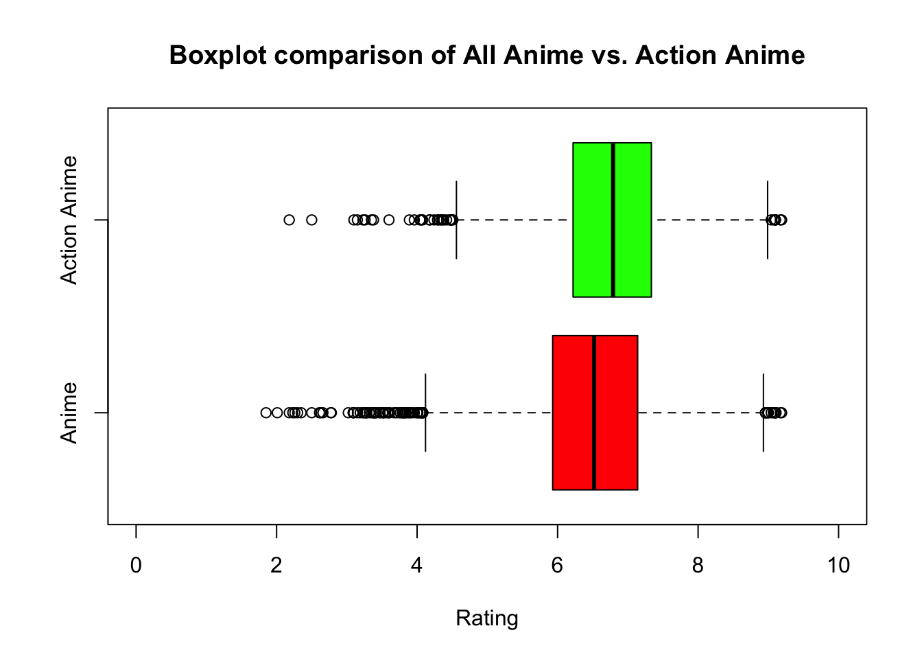
17.7 Run a Two Sample T-Test.
Based on the boxplots, it looks like there’s a difference. Action animes appear to be rated higher than the rest. That means:
Our null hypothesis is that there is no difference between the two averages, so u1 - u2 =0.
Our alternative hypothesis is that there is a difference between two averages, specifically that the average rating for all animes is lower than the average rating for action animes.
Set the alternative hypothesis to be that the true average score of all animes is LOWER than the true average score for action animes.
action_t_test <- t.test(anime_score, action_anime_score, alternative= "less", var.equal=TRUE)View the results.
##
##  Two Sample t-test
##
## data:  anime_score and action_anime_score
## t = -14, df = 15731, p-value <2e-16
## alternative hypothesis: true difference in means is less than 0
## 95 percent confidence interval:
##     -Inf -0.2125
## sample estimates:
## mean of x mean of y
##     6.510     6.751
Wow! There’s a serious difference. Look at the p-value for that. Now we need to graph this.
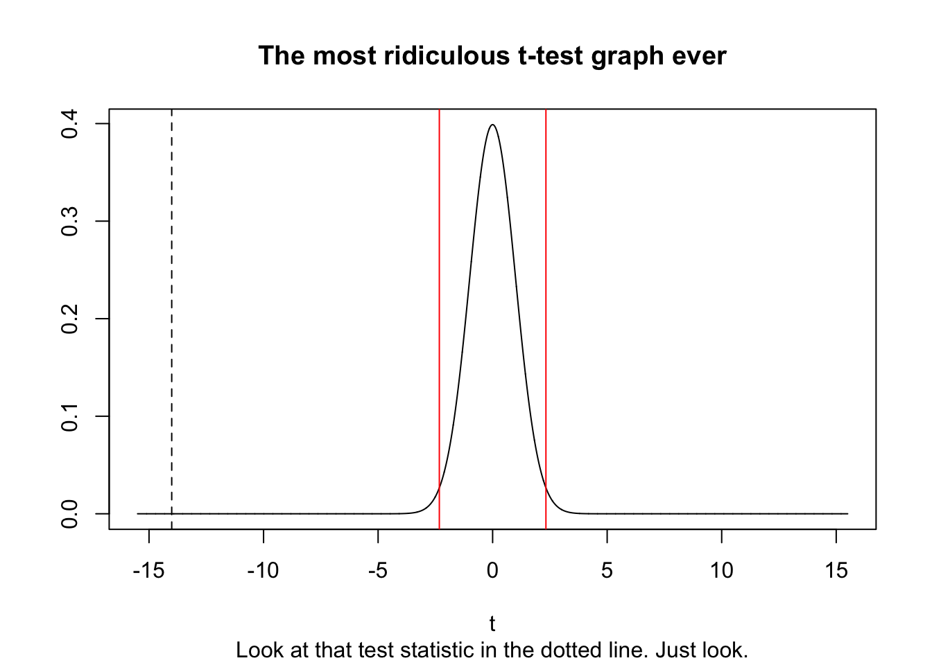
17.8 Graph the t-distribution and test statistic.
Let’s start by:
storing the degrees of freedom in a variable called action_t_test.
creating an x-axis and store it as a variable called t_d_st_x_axis. This is the equivalent of drawing tick marks everywhere on a graph, but a ton of tick marks. We’re making a huge sequence 10^4 numbers long (so 10000 numbers) between -15.5 and 15.5. This helps fit in my massive test statistic of -14.34
action_t_test_df<- length(anime_score) +length(action_anime_score) -2 #Recall how to calculate degrees of freedom.
t_dist_x_axis<- seq(-15.5, 15.5, length= 10^4)
Finally, plot. Notice here that for plot():
the x-value is t_dist_x_axis
the y-value is dt(t_dist_x_axis, df=action_t_test_df). This generates a t-value for every value in t_dist_x_axis, so basically f(x), with the degrees of greedom we set earlier.
plot(t_dist_x_axis, dt(t_dist_x_axis, df=action_t_test_df),
     type='l',
     xlab='t',
     ylab='',
     main="The most ridiculous t-test graph ever",
     sub="Look at that test statistic in the dotted line. Just look.")
I want to show how ridiculous this is. We’re going to store the critical t* value of 0.01 in it’s own variable, and plot that with red lines.
crit_t_value_0.01<- qt(0.01, df=action_t_test_df)
abline(v=crit_t_value_0.01, col='red')
abline(v=-crit_t_value_0.01, col='red')
Finally, plot the test statistic, using a dotted line.
abline(v=action_t_test$statistic, lty=2)