13 1️⃣『』 One Sample t-Interval for \(\mu\)
13.1 The t-distribution
Proportions= Normal Distribution (z-distribution)
Confidence Intervals for a population proportion \(p\) are based on z-values from the standard Normal distribution.
Proportions are really simple to work with, because they’re always standardized—the largest decimal is 1, and the smallest is 0. This means that we don’t have to worry about the spread of the population as much.
Means= \(t\)-distribution
Means can take any value—they could be negative, they could be 78, they could be 10,000. As a result, the sampling distribution for means naturally has a larger spread— this means that the sampling distribution is no longer normal.
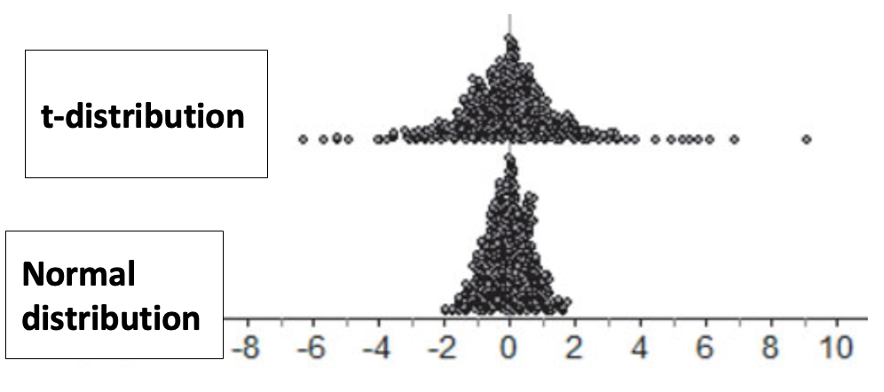
When we only know the sample’s standard deviation \(s_x\)—so not the population standard deviation \(\sigma\)—the distribution takes on a new shape called the t-distribution. You can see a comparison above.
The t-distribution has a much larger spread than the normal distribution does—this is to account for the naturally larger spread that sample means would have.
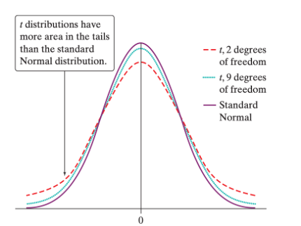
The \(t\)-distributions are a family of symmetric, bell-shaped distributions that are centered at 0, but whose spread is determined by its degrees of freedom. The area of those tails depends on the degrees of freedom the sampling distribution has. The larger the sample, the closer the t-distribution will get to the Normal distribution. The smaller the sample, the greater its varability, and so the t-distribution compenstates by adding more area in its tails.
When we talk about z-scores within the t-distribution (e.g. how many standard deviations a data point is away from the mean), we still use the same formula, but we now call them t-values, to differentiate them from the Normal distribution.
13.1.1 Distributions Calculator
Below is an app that calculates the areas of different distributions. Use the normal distribution, keep the mean and sd the same, but slide \(a\) around to examine the area underneath each tail.
Then, change to the \(t\)-distribution and investigate the area under the tail now. Change the degrees of freedom until you think you know what is going on.
13.2 Finding areas under the \(t\)-distribution
Just like how in 10.3.2 we used pnorm() to find areas given a \(z\)-score, and qnorm() to find \(z\) given a area, we can use pt() and qt() to find the t-distribution.
|
Find Area, given \(z\) or \(t\) |
Find \(z\) or \(t\), given Area |
|
|---|---|---|
| Normal (\(z\)) |
pnorm()
|
qnorm()
|
| \(t\) |
pt()
|
qt()
|
In both cases, R will always calculate the cumulative area starting from the left of the distribution.
13.3 One Sample Confidence Interval for \(\mu\)
Confidence Intervals for a population mean \(\mu\) use a t-distribution with \(n-1\) degrees of freedom.
Example: Biologists studying the healing of skin wounds measured the rate at which new cells closed a cut made in the skin of an anesthetized newt. Here are data from a random sample of 18 newts, measured in micrometers (millionths of a meter) per hour:
29 27 34 40 22 28 14 35 26 35 12 30 23 18 11 22 23 33
Calculate and interpret a 95% confidence interval for the mean healing rate µ.
13.3.1 State
We want to construct a One Sample Confidence Interval of the mean number of closed skin wounds in newts, with 95% confidence.
newts <- c(29, 27, 34, 40, 22, 28, 14, 35, 26, 35, 12, 30, 23, 18, 11, 22, 23, 33)

paste("Mean: ", mean(newts), "SD:", sd(newts), "n:", length(newts), sep= " ")
## [1] "Mean: 25.6666666666667 SD: 8.32430883900032 n: 18"So \(\bar{x} = 25.67\), \(s_\bar{x}= 8.324\), and \(n=18\).
13.3.2 Plan: Check for Conditions
There are three conditions you need to check for:
Random: The sample must be a random sample. This diminishes sampling bias.
Normal: \(n \ge 30\). This generally helps us fulfill the central limit theorem, so the sampling distribution of \(\bar{x}\) is approximately Normal. This number should be an integer, since it represents counts in the sample.
However, the \(t\)-distribution is what we call a robust distribution. Even if our sample size is less than 30, we can still proceed with our analysis provided the following:
Sample size less than 15: Use \(t\) procedures if the data appear close to Normal (roughly symmetric, single peak, no outliers). If the data are clearly skewed or if outliersa re present, do not use \(t\).
Sample size at least 15: The \(t\) procedures can be used except in the presence of outliers or strong skewness.
Sample size greater than 30: The \(t\) procedures can be used even for clearly skewed distributions when the sample is larger than 30.
- Independent (10% Condition): The number of successes (observational units in \(\bar{x}\)) and the number of failures (observation units not in \(\bar{x}\)) must be less than 10% of the population.
Random: Stated that this is a random sample of 18 newts. ✅
Normal: \(n \ngeq 30\), so we must look at the histogram of our data. ✅
hist(newts)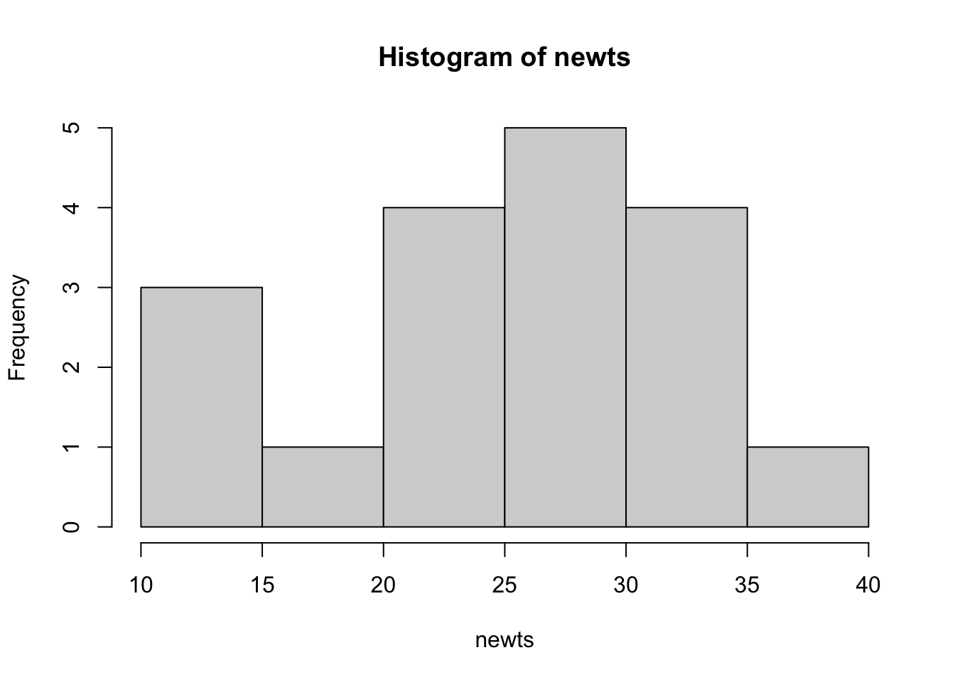
Since our sample size is at least 15 but less than 30, we need to check for any outliers or strong skewness. The histogram does not appear to show either, so we pass the Normal condition.
- Independent: \(18 * 10= 180\). It is reasonable to assume that there are more than 180 newts in the total population being sampled, so we pass this condition. ✅
Since we pass all three conditions, we can continue.
13.3.3 Do
Let’s do this manually first. Recall the formulas for a Confidence Interval and the Margin of Error.
\[\text{C.I.}= \bar{x} \pm \text{Margin of Error}\] \[= \bar{x} \pm t^*(\text{Standard Error})\]
Recalling what we learned in 11.4, we can substitute that Standard Error formula with the standard deviation of the sampling distribution, size \(n\):
\[\text{C.I.}= \bar{x} \pm t^*(\frac{s_\bar{x}}{\sqrt{n}})\]
DEFINITION: Standard error of the sample mean
The standard error of the sample mean x is \(\frac{s_\bar{x}}{\sqrt{n}}\) , where s_{x} is the sample standard deviation. It describes how far \(\bar{x}\) will be from \(\mu\), on average, in repeated SRSs of size \(n\).
- Find \(t^*\). Since our confidence level is 95%, that means we’re solving for the area outside of the middle 95% of the \(t\) distribution, with \(n-1= 18-1=17\) degrees of freedom.
Since \(t\) is symmetric, that means 2.5% is on either end of the tail. 95%+2.5% means we will solve for the 97.5th percentile.
qt(0.975, df= 17)## [1] 2.11Our \(t^*\) value is 2.11.
- Solve for the Margin of Error:
Mathematically:
\[ \text{Margin of Error}= \\ 2.11 * \frac{8.324}{\sqrt{18}} \\= 4.14 \]
Finally, we can create a 95% confidence interval.
#Lower Bound
25.667 - moe
## [1] 21.53
#Upper Bound
25.667 + moe
## [1] 29.81\[ \text{95% CI}= \bar{x} \pm \text{M.o.E}= 25.667 \pm 4.14 = [21.53, 29.81]\]
Fortunately, R does have a function that creates the confidence interval automatically, using the t.test function:
t.test(newts, conf.level=0.95)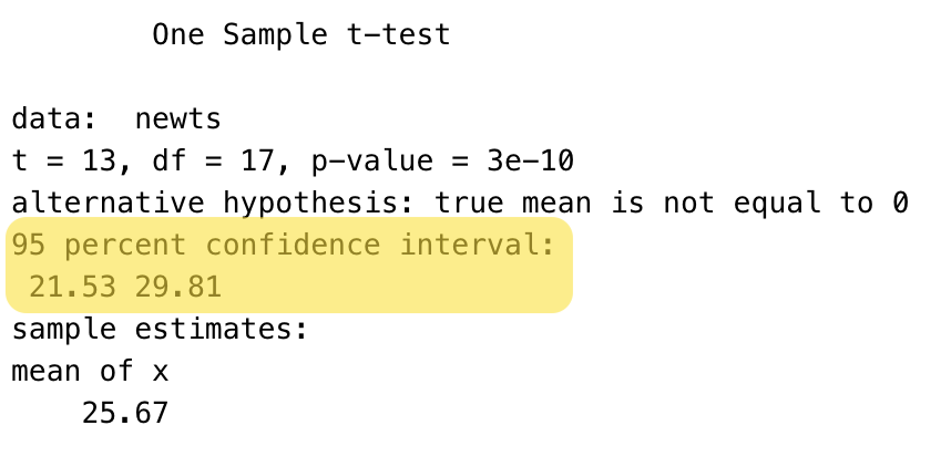
Ignore the other output for now– we will save that for the next chapter.
13.3.4 Conclude
We are 95% Confident that the interval from 21.53 wounds to 29.31 wounds captures the true mean number of closed skin wounds in newts.
You must always use context. Failure to do so would mean lost points.
Regardless of whether you calculate the interval by hand, R, or the TI-84, you must complete the State, Plan, and Conclude portions as shown. Failure to do so results in lost points.