14 1️⃣ One Proportion Z-Test for Proportions
14.1 Conceptually: Significance Testing= Quantifying Sussiness
The basketball team at a state university claims that each of their players makes 80% of their free throw shots. Do you think that the team actually can make 80% of their free throw shots, or are they just flexing? To test this claim, we’ll ask a player from the team to shoot free throws.
Ask a State University player to shoot free throws by clicking SHOOT. You can get more data by clicking Shoot repeatedly. Do the data appear to agree with the 80% claim or to give evidence against it? When you are satisfied, click “Show true probability” to see the truth for this player. Click NEW SHOOTER to test a different player, who may have a different free throw percent.
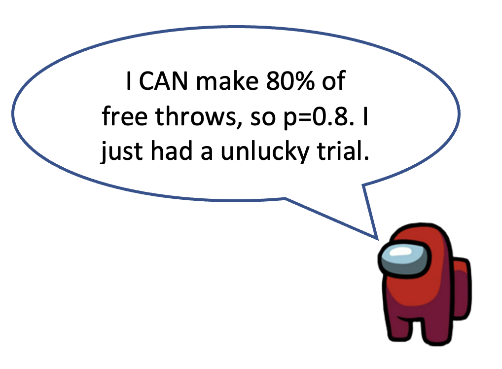
Suppose we test out another player—Player #3, and he makes 32 out of the 50 free throws that we give him. His sample proportion of made shots is \(\hat{p}=\frac{32}{50}=0.64\). What can we conclude about the player’s claim to 80% based on this one sample?
The answer is: not much. If he tells you that he was just having a bad day, or he’s just having bad luck, you can’t call him out on his lies, because you have a single sample. A single sample, as we already know, is not enough, because of sampling variability. How do we prove that he’s not simply having bad luck, but is just untalented?
When we take the evidence (\(\hat{p}=0.64\)) and weight it against a claim (that \(p=0.8\)), consider that there are only two explanations:
The player’s claim is correct (\(p=0.8\)), and by extraordinary bad luck, a very unlikely outcome occurred.
The population proportion is actually less than 0.8, so the sample result is not an unlikely outcome.
We know that the chance outcome of an unlucky sample is non-zero– that it can happen. The trick to proving the basketball player wrong is quantifying how unlikely he could’ve had a bad day, assuming he’s telling the truth. Assuming \(p=0.8\) is true, how likely could we have gotten \(\hat{p}=0.64\)? This is a significance test.
We can create a simulation of 50 free throws with 400 trials, assuming that the probability is true. Since we know our simulation was carried out truly by chance, we have a measurable way to outline how probable the player would’ve made 0.64 of shots.
bball_0.8 <- c(rep(1, times=40), rep(0, times=10))
simul_400_trials_50n<- replicate(400, sample(bball_0.8, 50, replace=TRUE))
results_simul_400_trials_50n<- colSums(simul_400_trials_50n) /50
hist(results_simul_400_trials_50n)

stripchart(results_simul_400_trials_50n, method = "stack",
           offset = .4,
           at = 0,
           pch = 19,
           col = "steelblue",
           main = "Results of 400 trials with 50 shots each",
           xlab = "Proportion made")
abline(v=0.64, col="red", lty=2)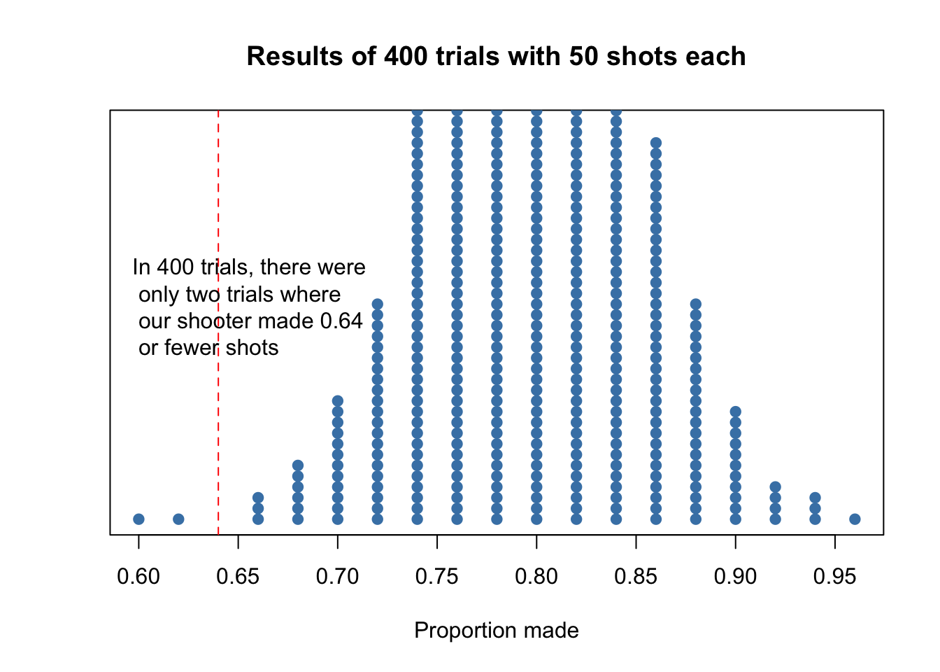
FIGURE 14.1: In 400 simulations, there were only two trials where our shooter got such an unlucky phat.
In our simulation, there were only 2 trials out of 400 that the player would’ve made 64% of his shots or less. Based on this simulation, our estimate of this probability is \(\frac{2}{400}=0.005\). The observed statistic, \(\hat{p}=\frac{32}{50}=0.64\), is so unlikely if the actual parameter value is p=0.8, that it give convincing evidence that the player’s claim is not true.
Explanation 1 might be correct—he could’ve just been unlucky. But the probability that such a result could’ve occurred just by chance is so small (less than \(\frac{1}{100}\)) that we are quite confident that Explanation 2 is right.
The process for significance tests is very similar to confidence intervals– we will use State, Plan, Do, and Conclude.
14.2 One Proportion \(Z\)-Test
A One-Proportion Z-Test is, frankly, the most useless significance test. However, we teach it because it is a good stepping stone to the other significance tests. Here’s the example problem:
A state’s Division of Motor Vehicles (DMV) claims that 60% of teens pass their driving test on their first attempt. An investigative reporter examines an SRS of the DMV records for 125 teens: 66 of them passed the test on their first try.
Is this good evidence that the DMV’s claim is incorrect? Carry out a test at the at the \(\alpha = .05\) significance level to help answer this question.
14.2.1 State
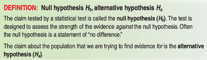
Assuming the statement is true is called the Null Hypothesis. It assumes that there is no difference between the claimed parameter (true proportion), and the sample proportion we measure.
The Alternative Hypothesis is that there is a difference between the claimed parameter, and the sample proportion we measure. In this case, it means the statistic we measured is so significantly different from the assumed “true claimed parameter,” that it simply couldn’t have happened by chance. In this case, we have good evidence that the claim about the proportion is false.
In this case, the claim from the DMV is that 60% of their teens pass the driving test on the first try. Our sample proportion is \(\hat{p}= \frac{66}{125}= 0.528\), which becomes evidence for or against the DMV’s claim that \(p=0.6\). Is \(\hat{p}= 0.528\) so significantly different from the claim of \(p=0.6\), that it becomes evidence against the DMV’s claim?
Given that our sample proportion is lower than the claim, we suspect that the true proportion is lower than 60%, so we set our alternative hypothesis appropriately, like below.
| Hypothesis | Meaning |
|---|---|
| \(H_0: p = 0.60\) | Our sample proportion falls within the realm of chance, and isn’t THAT different from the claim. We have no evidence that their claim is likely suss. |
| \(H_a: p<0.60\) | Our sample proportion is so different from what the company claims that \(\hat{p}\) is enough evidence to show their claim is likely suss. We suspect that the true proportion of teenagers passing the DMV test is lower. |
… where \(p\) is the true, long-run proportion of teenagers who take the DMV and pass the DMV test on the first try.
The null and alternative hypothesis are ALWAYS about your population parameter, which is \(p\). It is NEVER about your sample statistic, because you don’t need to test the sample statistic. You already have it. Remember the goal is always to use your sample statistic to make inferences about the larger population.
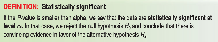
Finally, we want to state a red line for determining whether something is suss. If the probability that we would’ve gotten that measured statistic is less than ______, then we had enough evidence to reject \(H_0\) in favor of \(H_a\). This threshold is our significance level, called alpha.
By tradition, \(\alpha=0.05\). That means that if we calculate that the probability of getting \(\hat{p}=0.528\) by pure chance was less than 0.05, we can say the company is suss.
14.2.2 Plan
The conditions remain the same three as 12.3.2.
Random: The sample of 125 teens was randomly selected. ✅
Normal: To use a Normal approximation for the sampling distribution of \(\hat{p}\), we need both \(np\) and \(n(1-p)\). Since we don’t know \(p\), we use \(\hat{p}\) instead.
We check that \(np = 125(0.528)= 66 \ge 10\) and \(n(1-p) = 125(1-0.528) =59 \ge 10\). Since both are greater than 10, we fulfill this condition. ✅
Independent: If our is sample size \(n=125\) is exactly 10% of the population, then that means the smallest possible population size is \(10*125=1250\). Given that we know that there are way more than 1250 students taking a road test every year, it is reasonable to assume that our sample size is less than 10% of the population. ✅
Since we pass all three conditions, we can continue with our significance test.
14.2.3 Do
We’ll first manually do the z-test.
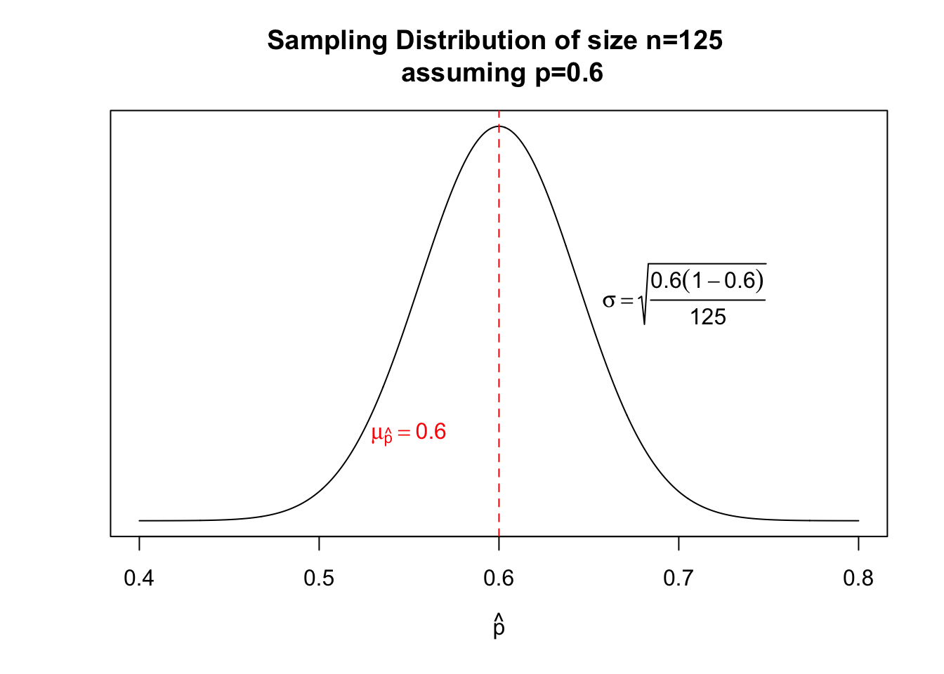
Assuming that the null hypothesis is true, that means that there exists a sampling distribution of size \(n=1029\) centered at \(p=0.60\) with a standard deviation of \(\sqrt{\frac{p(1-p)}{n}} = \sqrt{\frac{0.6(1-0.6)}{125}} = 0.0438178\)
Where would our sample proportion exist on this sampling distribution? Not only is \(\hat{p}=0.528\) left of the center, but we should also be able to derive a z-score of how many standard deviations our sample \(\hat{p}\) is from the mean. This number is called the test statistic.
Definition: Test Statistic
A test statistic measures how far a sample statistic diverges from what we could expect if the null hypothesis \(H_0\) were true, in standardized units. That is,
\[\text{test statistic} = \frac{\text{statistic} - \text{parameter}}{\text{stadard deviation of the statistic}}\]
To calculate this test statistic, let’s plug it into our formula, knowing that the null hypothesis parameter (the claim) \(\mu_0 = 0.6\), the sample statistic is \(\hat{p}=0.528\), and the standard deviation was \(\sqrt{\frac{0.6(1-0.6)}{125}} = 0.0438178\).
\[\text{test statistic}= \frac{0.528 - 0.6}{0.0438178}= -1.643167\]
This means that, if \(H_0\) were true, the sample we received was 1.64 standard deviations below the mean. We can now use pnorm() to derive that probability we would’ve received this score, assuming the DMV is telling the truth.
pnorm(-1.643167)## [1] 0.05017This number is called the p-value.
Definition: P-Value
The probability, computed assuming \(H_0\) is true, that the statistic (such as \(\hat{p}\) or \(\bar{x}\)) would take a value as extreme as or more extreme than the one actually observed is called the P-Value of the test. The smaller the P-Value, the stronger the evidence against \(H_0\) provided by the data.
If the DMV’s claim is true, then that means we would have a 5.01% chance of getting our sample \(\hat{p}=0.528\) or lower. Is this enough to prove that the DMV is not telling the truth?
14.2.4 Conclude
Fortunately, you already set a threshold for whether you would reject, or fail to reject: the alpha value \(\alpha\).
If P-Value > \(\alpha\), you fail to reject \(H_0\). You do not have sufficient evidence to reject the null hypothesis, and therefore we could’ve gotten our different sample proportion by chance, due to sampling variability.
If P-Value < \(\alpha\), you reject \(H_0\). You have sufficient evidence to reject the null hypothesis, and your sample statistic is significantly significant from the claim in the null hypothesis.
Based on our p-value, even though it is very close to 0.05, it is still slightly above 0.05. Because of this, we:
Fail to reject \(H_0\). There is not sufficient evidence that the first time passing rate of teenagers taking the driving test is less than 60%.
You NEVER “accept” the null hypothesis or alternative hypothesis. You either reject, or fail to reject the null hypothesis. Just because you have strong evidence against the null hypothesis does not necessarily mean that your alternative is true.
14.3 In R
You can use the prop.test() command that was referenced in 12.4. We include two extra parameters: p= and alternative=, were p= is the null hypothesis probability, and alternative= is the alternative hypothesis.
prop.test(x=66,
          n=125,
          p=0.6,
          alternative="less",
          correct=FALSE)
##
## 1-sample proportions test without continuity
## correction
##
## data: 66 out of 125, null probability 0.6
## X-squared = 2.7, df = 1, p-value = 0.05
## alternative hypothesis: true p is less than 0.6
## 95 percent confidence interval:
## 0.0000 0.6001
## sample estimates:
## p
## 0.528The alternative= parameter takes on three possible arguments:
greaterorless: these are where we believe the true \(p\) value is less than, or greater than, the null hypothesis. These are One-Sided Tests, because we only calculate the area under the curve from one side of the sampling distribution.two-sided: this is where we believe the true \(p\) value is either greater than or less than the null. We have no idea which way it goes, so out of caution, we examine both p-values. These are Two-Sided Tests, because we only calculate the area under the curve from both sides of the sampling distribution at the same time. If you do not specify your alternative hypothesis, R will default to this parameter.
Again, regardless of whether you calculate the interval by hand, R, or the TI-84, you must complete the State, Plan, and Conclude portions as shown. Failure to do so results in lost points.