7 🎲 Sampling and Probability
7.1 An overview on probability
While a chance process is impossible to predict in the short term, if we observe more and more repetitions of any chance process, the proportion of times that a specific outcome occurs approaches a single value. This is called The Law of Large Numbers.
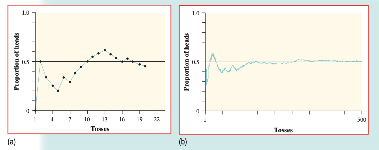
FIGURE 7.1: (a) The proportion of heads in the first 20 tosses of a coin. (b) The proportion of heads in the first 500 tosses of a coin.
Above is the cumulative proportion of tosses for a fair coin. The previous example confirms that the probability of getting a head when we toss a fair coin is 0.5. Probability 0.5 means “occurs half the time in a very large number of trials.” That doesn’t mean that you are always guaranteed 50% heads and 50% tails for any number of tosses!
The Law of Large Numbers, therefore, never guarantees a specific outcome when we observe a chance process—rather, it points out that there the proportion trends towards the value that we predict for the chance process.
- Empirical means something based in observation and experience, rather than theory or logic.
- “Empirical probabilities come from carrying out a simulation and recording the results. The probability of each event and outcome was the observed relative frequency from the simulation. You found empirical probabilities from Random Babies and Pass the Pigs activity.”
- Theoretical means something based in logic, rather than observation.
- Theoretical probabilities come from constructing a sample space.
The sample space is a list of all possible outcomes. - For example, when you toss a die, there are six possible outcomes. If the die is fair, then are all equally likely to occur. So, the sample space S for a fair die is \[S= {1,2,3,4,5,6}.\]
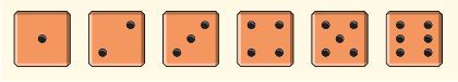
FIGURE 7.2: All possibilities of a six-sided die.
An event is a subset of a sample space. - For example, the event of “tossing a prime number” in our dice example is the set {2,3,5}. In a sample space with equally likely outcomes, the probability of an event P(E) is \[P(E)=\frac{\text{Number of Outcomes in the Event}}{\text{Total Number of Outcomes in the Sample Space}}\]
So, the theoretical probability of tossing a prime number is \(\frac{1}{2}\).
Finally…
All events have probabilities between 0 and 1, inclusive.
The probability of an impossible event is 0.
The probability of a certain (guaranteed to happen) event is 1.
7.2 Performing Simulations
7.2.1 Carrying out simulations in R using sample()
Carrying out a simulation in R is very easy– much easier to do than using a chance process like dice, a random number generator, and so forth. Like all those other processes though, you must first construct the sample space.
Let’s simulate the roll of dice. First, I’ll create a new vector that counts from 1 to 6, and store it as dice.
dice <- 1:6When you run the sample() command, R effectively selects an element randomly from the vector– almost like you placed each vector element on its own index card, and you pull one out. This behavior cannot be changed.
sample(dice,
       size = 5,
       replace=FALSE)
## [1] 3 1 4 5 6Here are the parameters, explained:
-
dice=is the vector that we are sampling from. -
size=is the number of times that we are sampling from this vector. This is the sample size. -
replace=tells R whether to sample for replacement.FALSEmeans sampling without replacement.FALSEis the default setting; if you do not specifyreplace=, it will assumeFALSE. What that means is that once R has selected that element, it will exclude that element from the second selection.
As you can see, it means that every face of the die is selected exactly once. While this works for 6 index cards labeled 1 to 6, it doesn’t make sense for dice. We know for a fact that numbers can be repeated on a dice.
Replacing with replace=TRUE allows us to properly replicate the chance process of rolling a dice. Here, we roll the dice 7 times. Notice that some numbers repeat.
sample(dice,
       size = 5,
       replace=TRUE)
## [1] 5 1 1 2 4If you kept replace=FALSE, and selected a size= that was larger than the number of elements in dice, you get an error. If you sample without replacement, and you exclude any elements that have already been selected, you select all elements exactly once with size=6. There are no more elements beyond 6.
sample(dice,
       size = 7,
       replace=FALSE)
## Error in sample.int(length(x), size, replace, prob): cannot take a sample larger than the population when 'replace = FALSE'
7.2.2 Sampling from a table using slice_sample()
Let’s return to our periodic_table data from the previous chapter. Given that each row represented an element (in our case, an observational unit), we can use the slice_sample() function to select different elements at random.
slice_sample(periodic_table, n=5, replace=FALSE)## # A tibble: 5 × 22
## atomic_number symbol name name_origin group period block
## <dbl> <chr> <chr> <chr> <dbl> <dbl> <chr>
## 1 116 Lv Live… Lawrence L… 16 7 p
## 2 109 Mt Meit… Lise Meitn… 9 7 d
## 3 82 Pb Lead English wo… 14 6 p
## 4 30 Zn Zinc the German… 12 4 d
## 5 14 Si Sili… from the L… 14 3 p
## # … with 15 more variables: state_at_stp <chr>,
## # occurrence <chr>, description <chr>,
## # atomic_weight <dbl>, aw_uncertainty <dbl>,
## # any_stable_nuclides <chr>, density <dbl>,
## # density_predicted <lgl>, melting_point <dbl>,
## # mp_predicted <lgl>, boiling_point <dbl>,
## # bp_predicted <lgl>, heat_capacity <dbl>, …The advantage here over using sample(1:118, 5) (since there are 118 rows, and therefore chemical elements, in this table), is that you don’t need to choose the data associated with that observation all over again. You can now work with an columns associated with each sampled row, instead of manually selecting it.
Here’s another example using 5.3 to do more advanced sampling. In our ChickWeight scenario, we couldn’t just sample each row first, because each row represented a single observation of a chicken by Day. Let’s say I want to sample 5 chickens, on Diet 1, on Day 18:
chicken_sample <- ChickWeight %>%
  dplyr::filter(Time==18, Diet==1)

chicken_sample<- slice_sample(chicken_sample, n=5, replace=FALSE)

chicken_sample
## weight Time Chick Diet
## 1 248 18 14 1
## 2 199 18 5 1
## 3 160 18 6 1
## 4 184 18 11 1
## 5 185 18 12 1Now, we can derive a mean weight from our chicken_sample with mean(chicken_sample$weight).
7.2.3 Repeating Trials
R cannot do everything for us. At every point when we design a simulation, we must make choices.
sample(dice,
       size = 5,
       replace=TRUE)
## [1] 2 5 4 2 5The code above can be interpreted as taking a single dice, and rolling it five times. That means there are 5 trials with 1 observation in each trial.
But an alternative interpretation of the code above is that this is 1 trial where we threw 5 dice at once, simultaneously. In this case, it means that, if we want 5 trials, we would have to run the code over and over.
If we were to simulate the probability of throwing multiple dice at once, over multiple trials, we would need to run the sample() command over and over. Manually running the command isn’t practical, so we use the replicate() function instead.
##      [,1] [,2] [,3] [,4] [,5] [,6] [,7] [,8] [,9] [,10]
## [1,]    1    4    6    3    1    5    1    1    4     2
## [2,]    3    3    5    6    2    6    4    4    3     2
## [3,]    1    3    1    4    5    2    1    6    4     5
## [4,]    6    2    5    5    5    2    2    5    2     2
## [5,]    4    2    5    1    5    1    6    5    1     3
simul_5dice_10trials represents the simulation of throwing five dice per trial, over ten trials. Therefore, each column represents one trial, and each element in the column represents the result of that dice.
7.3 Tabluating using Two-Way Tables
As we learned in @(table), we can use the table() function to return the counts of a single quantitative variable. Here’s an example with the diamonds dataset, built into R, which contains the prices and attributes of 54,000 diamonds.
head(diamonds)## # A tibble: 6 × 10
## carat cut color clarity depth table price x y
## <dbl> <ord> <ord> <ord> <dbl> <dbl> <int> <dbl> <dbl>
## 1 0.23 Ideal E SI2 61.5 55 326 3.95 3.98
## 2 0.21 Premium E SI1 59.8 61 326 3.89 3.84
## 3 0.23 Good E VS1 56.9 65 327 4.05 4.07
## 4 0.29 Premium I VS2 62.4 58 334 4.2 4.23
## 5 0.31 Good J SI2 63.3 58 335 4.34 4.35
## 6 0.24 Very G… J VVS2 62.8 57 336 3.94 3.96
## # … with 1 more variable: z <dbl>The diamonds dataset includes multiple cateogorical variables that describe the quality of a diamond, including cut, color, and clairty. It would be very easy to tabulate each variable at once, by selecting each column as a vector.
table(diamonds$cut)##
## Fair Good Very Good Premium Ideal
## 1610 4906 12082 13791 21551
table(diamonds$color)##
## D E F G H I J
## 6775 9797 9542 11292 8304 5422 2808We can go further. What if I wanted to know how many diamonds were both cut== "Ideal"and color== "E"? In this case, we can pass both variables into R so it cross-tabulates the data for us.
table(diamonds$cut, diamonds$color)##
## D E F G H I J
## Fair 163 224 312 314 303 175 119
## Good 662 933 909 871 702 522 307
## Very Good 1513 2400 2164 2299 1824 1204 678
## Premium 1603 2337 2331 2924 2360 1428 808
## Ideal 2834 3903 3826 4884 3115 2093 8967.3.1 Deriving Marginal probabilities/ proportions from a two-way table
Now that we have the counts, it is easy for R to find the marginal probabilities from the table. Just pass the entire table() output into the proportions command.
proportions(table(diamonds$cut, diamonds$color))##
## D E F G H
## Fair 0.003022 0.004153 0.005784 0.005821 0.005617
## Good 0.012273 0.017297 0.016852 0.016148 0.013014
## Very Good 0.028050 0.044494 0.040119 0.042621 0.033815
## Premium 0.029718 0.043326 0.043215 0.054208 0.043752
## Ideal 0.052540 0.072358 0.070931 0.090545 0.057749
##
## I J
## Fair 0.003244 0.002206
## Good 0.009677 0.005692
## Very Good 0.022321 0.012570
## Premium 0.026474 0.014980
## Ideal 0.038802 0.016611