17 One-Way ANOVA
17.1 Comparing Several means: Hummingbirds and Tropical Flowers
Ethan Temeles and W. John Kress of Amherst College studied the relationship between varieties of the tropical flower Heliconia on the island of Dominica and the different species of hummingbirds that pollinate the flowers. Over time, the researchers believe, the lengths of the flowers and the forms of the hummingbirds’ beaks have evolved to match each other. If that is true, flower varieties pollinated by different hummingbird species should have distinct distributions of length.
The table below gives length measurements (in millimeters) for random samples of three varieties of Heliconia, each pollinated by a different species of hummingbird. Do the three varieties display distinct distributions of length? In particular, do the mean lengths of their flowers differ?
For the flower data, I made a CSV file from the textbook data, and then imported it into R.
| H. bihai | H. caribea red | H. caribea yellow |
|---|---|---|
| 47.12 | 41.90 | 36.78 |
| 46.75 | 42.01 | 37.02 |
| 46.81 | 41.93 | 36.52 |
| 47.12 | 43.09 | 36.11 |
| 46.67 | 41.47 | 36.03 |
| 47.43 | 41.69 | 35.45 |
| 46.44 | 39.78 | 38.13 |
| 46.64 | 40.57 | 37.10 |
| 48.07 | 39.63 | 35.17 |
| 48.34 | 42.18 | 36.82 |
| 48.15 | 40.66 | 36.66 |
| 50.26 | 37.87 | 35.68 |
| 50.12 | 39.16 | 36.03 |
| 46.34 | 37.40 | 34.57 |
| 46.94 | 38.20 | 34.63 |
| 48.36 | 38.07 | NA |
| NA | 38.10 | NA |
| NA | 37.97 | NA |
| NA | 38.79 | NA |
| NA | 38.23 | NA |
| NA | 38.87 | NA |
| NA | 37.78 | NA |
| NA | 38.01 | NA |
In order for R to process the data, I need to convert the data from “wide” format to “long” format. I also need to let R know that each species should be treated as a “factor,” which means that it is a type of categorical variable (so I can sort out data based on Species) later on.
Flowers_long<- gather(Flowers, "Species", "Length", factor_key= TRUE)
Flowers_long<- na.omit(Flowers_long)
head(Flowers_long)| Species | Length |
|---|---|
| H. bihai | 47.12 |
| H. bihai | 46.75 |
| H. bihai | 46.81 |
| H. bihai | 47.12 |
| H. bihai | 46.67 |
| H. bihai | 47.43 |
| H. bihai | 46.44 |
| H. bihai | 46.64 |
| H. bihai | 48.07 |
| H. bihai | 48.34 |
| H. bihai | 48.15 |
| H. bihai | 50.26 |
| H. bihai | 50.12 |
| H. bihai | 46.34 |
| H. bihai | 46.94 |
| H. bihai | 48.36 |
| H. caribea red | 41.90 |
| H. caribea red | 42.01 |
| H. caribea red | 41.93 |
| H. caribea red | 43.09 |
| H. caribea red | 41.47 |
| H. caribea red | 41.69 |
| H. caribea red | 39.78 |
| H. caribea red | 40.57 |
| H. caribea red | 39.63 |
| H. caribea red | 42.18 |
| H. caribea red | 40.66 |
| H. caribea red | 37.87 |
| H. caribea red | 39.16 |
| H. caribea red | 37.40 |
| H. caribea red | 38.20 |
| H. caribea red | 38.07 |
| H. caribea red | 38.10 |
| H. caribea red | 37.97 |
| H. caribea red | 38.79 |
| H. caribea red | 38.23 |
| H. caribea red | 38.87 |
| H. caribea red | 37.78 |
| H. caribea red | 38.01 |
| H. caribea yellow | 36.78 |
| H. caribea yellow | 37.02 |
| H. caribea yellow | 36.52 |
| H. caribea yellow | 36.11 |
| H. caribea yellow | 36.03 |
| H. caribea yellow | 35.45 |
| H. caribea yellow | 38.13 |
| H. caribea yellow | 37.10 |
| H. caribea yellow | 35.17 |
| H. caribea yellow | 36.82 |
| H. caribea yellow | 36.66 |
| H. caribea yellow | 35.68 |
| H. caribea yellow | 36.03 |
| H. caribea yellow | 34.57 |
| H. caribea yellow | 34.63 |
Let’s follow the strategy we learned way back in Unit 1: use graphs and numerical summaries to compare the three distributions of flower length. Here are the summary statistics we will use in further analysis:
mean_and_sd<- Flowers_long %>%
  group_by(Species) %>%
  summarize(mean=mean(Length, na.rm=T),
            sd=sd(Length, na.rm=T))
mean_and_sd| Species | mean | sd |
|---|---|---|
| H. bihai | 47.60 | 1.2129 |
| H. caribea red | 39.71 | 1.7988 |
| H. caribea yellow | 36.18 | 0.9753 |
What do we see? The three varieties differ so much in flower length that there is little overlap among them. In particular, the flowers of bihai are longer than either red or yellow. The mean lengths are 47.6 mm for H. bihai, 39.7 mm for H. caribaea red, and 36.2 mm for H. caribaea yellow. Are these observed differences in sample means statistically significant? We must develop a test for comparing more than two population means.
17.2 The F Test
We want to test the null hypothesis that there are no differences among the mean lengths for the three populations of flowers:
\(H_0:\mu_1 =\mu_2 =\mu_3\)
The alternative hypothesis is that there is some difference. That is, not all three population means are equal:
\(H_a\) : not all of \(\mu_1, \mu_2, \text{ and }\mu_3\) are equal
The alternative hypothesis is no longer one-sided or two-sided. It is “many-sided” because it allows any relationship other than “all three equal.”
For example, Ha includes the case in which m2 = m3 but m1 has a different value.
When the conditions for inference are met, the appropriate significance test for comparing means is the analysis of variance F test. Analysis of variance is usually abbreviated as ANOVA.
17.3 Check for Conditions
Now that we have stated our Null and Alternative Hypotheses, we can check for the four conditions required for One-Way ANOVA:
Random: Researchers took separate random samples of 16 bihaii, 23 red, and 15 Heliconia flowers.
Normal: We entered the data into R and made side by side boxplots. Although the distributions for the bihai and red varieties show some right-skewness, we don’t see nay strong skewness or outliers that would prevent the use of one-way ANOVA.
ggplot(Flowers_long, aes(x=Length, y=Species, fill=Species))+
  geom_boxplot(color="black")+
  labs(title= "Flower Lengths from Textbook")+
  geom_jitter(width=0.1) #This overlays a jittered dotplot on top of the boxplot.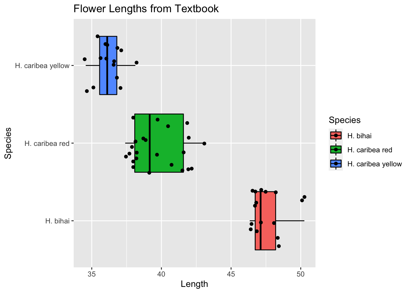
Independent: Researchers took independent samples of bihai, red, and yellow Heliconia. because sampling without replacement was used, there must be at least 10(16) = 160 bihai, 10(23) = 230 red, and 10(15) = 150 yellow flowers. This is pretty safe to assume.
Same SD: In a one-way ANOVA, you must check whether the largest sample SD divided by the smallest SD has a ratio less than 2. Our sample standard deviations are:
| Species | mean | sd |
|---|---|---|
| H. bihai | 47.60 | 1.2129 |
| H. caribea red | 39.71 | 1.7988 |
| H. caribea yellow | 36.18 | 0.9753 |
These standard deviations satisfy our rule of thumb that (largest SD)/ (smallest SD) is less than 2, so we can proceed.
Since we have satifised all 4 conditions, we can safely use ANOVA to compare the mean lengths of the three populations.
17.4 The F Distribution
The variances for three populations is naturally larger than the variance of two populations. Just like how two populations naturally have a larger variance, and thus requires the t-distribution (which has more “area” under the tails), we need to use a different distribution that takes into account this larger variance (which has even more “area” under the tails. This distribution is called the F-Distribution.
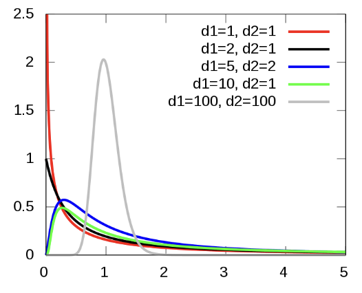
FIGURE 17.1: The F-Distribution
The F-distributions are a family of right-skewed distributions that take only values greater than 0. Above are some possible shapes. A specific F distribution is determined by the degrees of freedom of the numerator and denominator of the F statistic. When describing an F distribution, always give the numerator degrees of freedom first. Our notation will be F (df1, df2) for the F distribution with df1 degrees of freedom in the numerator and df2 degrees of freedom in the denominator. Interchanging the degrees of freedom changes the distribution, so the order is important.
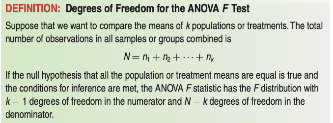
17.4.1 Finding the Degrees of Freedom for F
In the two earlier examples, we compared the mean lengths for three varieties of flowers,so k=3.The three sample sizes are n1 =16,n2 =23,and n3 =15. The total number of observations is therefore N = 16 + 23 + 15 = 54. The ANOVA F test has numerator degrees of freedom \[k - 1 = 3 - 1 = 2\] and denominator degrees of freedom \[N - k = 54 - 3 = 51\].
17.4.2 Understanding the F Statistic
Just like we had a test statistic in a two-sample t-test, we need something similar to tell us the distance the statistic is away from our Null Hypothesis. This distance is called the F Statistic.
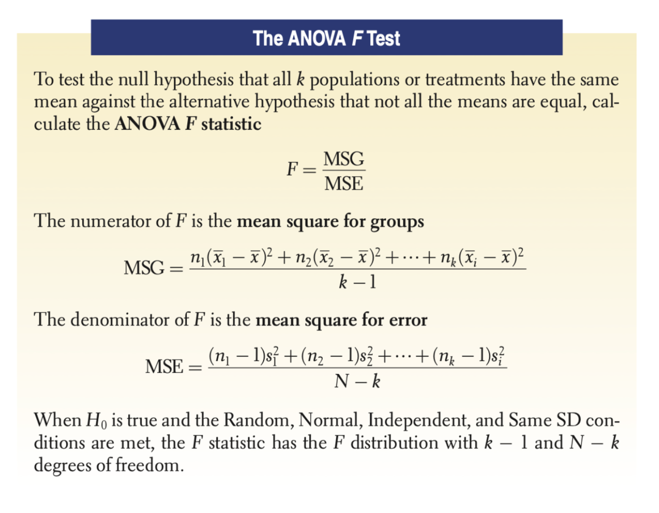
The F Statistic is calculated by doing:
\[ F= \frac{\text{variation among the sample means}}{\text{variation among individuals within the same sample}} \]
Specifically, the variation is calculated by dividing the Mean Square for Groups by the Mean Square for Error. The statistic is reproduced below, but you should know that you’d never have to do this by hand– R will do it all for you.
17.5 Conducting the one-way ANOVA
Of course, the previous pages gave you a very brief background of a one-way ANOVA test.
It turns out that conducting the test itself in R is very easy– R even calculates the degrees of freedom for you.
Flowers_long <- na.omit(Flowers_long)
anova.test <- aov(Length ~ Species, data=na.omit(Flowers_long))
summary(anova.test)
## Df Sum Sq Mean Sq F value Pr(>F)
## Species 2 1083 541 259 <2e-16 ***
## Residuals 51 107 2
## ---
## Signif. codes:
## 0 '***' 0.001 '**' 0.01 '*' 0.05 '.' 0.1 ' ' 1Looking at the P Value for Species, the one-way ANOVA Test tells us that there is a very significant difference between the average lengths of the 3 species. Thus, we reject the Null Hypothesis, and in favor of the Alternative Hypothesis that ther is a significant difference between the three species.
17.6 Conclude Pt. 2: Creating Tukey Post-Hoc Pairwise Comparisons
Knowing that there is a difference is often not enough– what if you want to know exactly which means were significantly different from each other? In this case, we’d have to conduct a two-sample t-test for every possible two means that we have, which could be irritating, especially if we are comparing many means with each other.
This is where a Tukey Post-Hoc Pairwise Comparison comes into play. The name sounds scary, but the following is true:
A guy named Tukey created this method.
“Post-Hoc” means “after the fact” in Latin. After knowing the fact that there is a difference among all three means from a one-way ANOVA, you can perform this procedure.
“Pairwise Comparision” means you compare two things with each other.
To perform the pairwise comparison, run the TukeyHSD() command on your anova.test model.
TukeyHSD(anova.test, conf.level=.95)## Tukey multiple comparisons of means
## 95% family-wise confidence level
##
## Fit: aov(formula = Length ~ Species, data = na.omit(Flowers_long))
##
## $Species
## diff lwr upr
## H. caribea red-H. bihai -7.886 -9.022 -6.750
## H. caribea yellow-H. bihai -11.417 -12.672 -10.163
## H. caribea yellow-H. caribea red -3.531 -4.689 -2.373
## p adj
## H. caribea red-H. bihai 0
## H. caribea yellow-H. bihai 0
## H. caribea yellow-H. caribea red 0You can also plot these results, as shown below:
#Margins will spill over, so you need to adjust these
par(mar=c(4, 13, 4, 4)+0.1)

plot(TukeyHSD(anova.test, conflevel=.95), las=1, col="blue")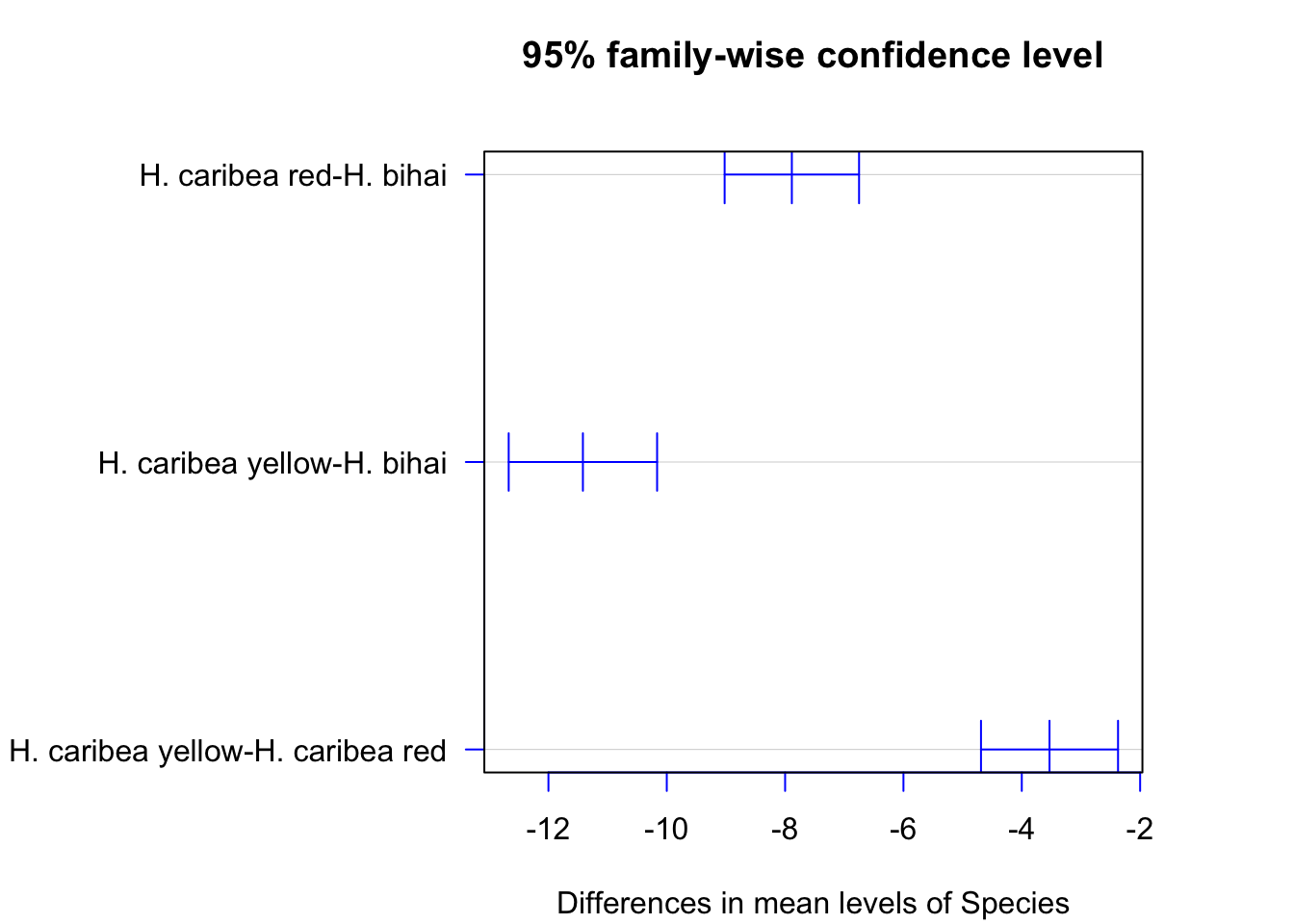
Notice that the x-axis doesn’t even include 0– our pairwise comparisons illustrate that all of the species are significantly different from each other in terms of mean length. Notice that none of the confidence intervals include 0 (what does that mean?).