1 📑 Vectors

taken from Ismay and Kennedy (2016) and Kane (2022).

1.0.1 Basic Commands

Before we get started, there are a few terms, tips, and tricks that you should know before getting started with R.

Functions: these perform tasks by taking an input called an argument and returning an output. Take a look at the example below.
```
sqrt(64)
```
```
## [1] 8
```

sqrt() is a function that gives us the square root of the argument. 64 is the argument. Therefore, the output should be 8. Try it for yourself in the console!

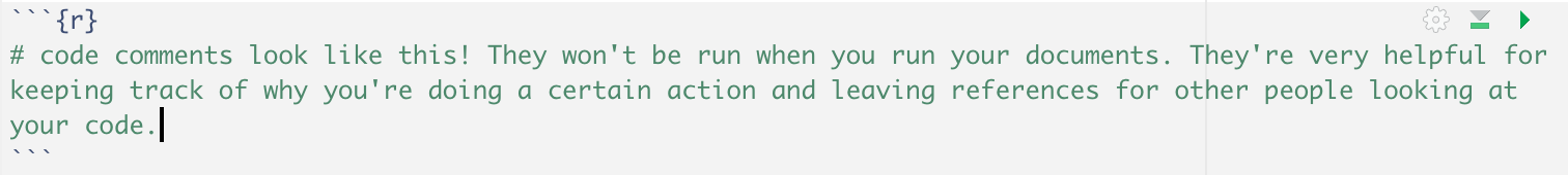
Help files: these provide documentation for functions and datasets. You can bring up help files by adding a ? before the name of the object then run this in the console. The boxplot command, for example, creates a boxplot. Run ?boxplot in the console and see what pops up.
Code comments: these are text placed after a # symbol. Nothing will be run after a # symbol, which is useful when you include comments in your code, as you always should. The image below shows what a code comment looks like.

Errors, warnings, and messages: these generally reported in a red font. When there is an error, the code will not run. Read (and/or Google) the message and try fix it. Warnings don’t prevent code from completing. For example, if you create a scatterplot based on data with two missing values, you will see this warning:
```
Warning message:
Removed 2 rows containing missing values (geom_point).  
```
Messages are similar. In both cases, you should fix the underlying issue until the warning/message goes away.

Remember: in the last chapter, we used the operator <- to store the number 9 into a variable called x. The operator <- is used in R to store literally any object as a variable, so it can be referenced later. We will be using <- in our programming.

Remember, you don’t store anything until you run the <- command. Check the top right pane in RStudio to verify that you stored the object.

1.1 Vector Overview

A vector is the most basic data object in R. It is essentially a list, and can take on different types. Even when you write a single value in R, it is considered a vector with a length of 1. So when you typed x <- 9, you have a vector called x with a length of 1, and that single element is 9.

In this class, we will only focus on character, double, and logical vectors.

A numeric vector, also called a double vector, is a vector that is entirely made of numbers. A vector that is entirely decimals is an integer vector, and you can specify to R that a number is an integer by adding L at the end– so 34L specifies the integer 34. The reasons behind this have to do with floating point arithmetic in computers, and we won’t get to the differences between these in this class.
Character vectors, on the other hand, stores any combination of letters and symbols. As soon as you include a character in any double vector, it will become a character vector.
Logical vectors store truth values TRUE and FALSE. They are useful when meeting a condition.

The str command allows us to see each vector type.

Press the “Run code” button to see this in action:

1.1.1 Concatenating Vectors

If you would like to list out many entries and put them into a vector object, you can do so via the c function. If you enter ?c in the R Console, you can gain information about it. The “c” stands for combine or concatenate.

Suppose we wanted a way to store four names:

friend_names <- c("Abram", "Bryant", "Colleen", "David", "Esther", "Jeremiah")
friend_names

## [1] "Abram"    "Bryant"   "Colleen"  "David"    "Esther"  
## [6] "Jeremiah"

You can see when friend_names is outputted that there are four entries to it. This is vector is known as a strings vector since it contains character strings. You can check to see what type an object is by using the class function:

class(friend_names)

## [1] "character"

Next suppose we wanted to put the ages of our friends in another vector, and their favorite number. We can again use the c function:

friend_ages <- c(34, 35, 32, 29, 30, 30)
friend_fav_number<- c(1, 2.17, 26, 7, 10, 9)
class(friend_ages)

## [1] "numeric"

And finally, an example of a logical vector:

lives_in_dc <- c(TRUE, FALSE, FALSE, TRUE, FALSE, TRUE)

Note that TRUE and FALSE must be in all caps for R to recognize that these are boolean (“truth”) values.

From a user’s perspective, there is not a huge difference in how these values are stored, but it is still a good habit to specify what class your variables are whenever possible to help with collaboration and documentation.

1.1.2 Using the seq() function

The most likely way you will enter character values into a vector is via the c function. Numeric values can be entered in a couple different ways. One is using the c function, as we saw above. Because numbers have a natural order, we can also specify a sequence of numbers with a starting value, an ending value, and the amount by which to increment each step in the sequence:

sequence_by_2 <- seq(from = 0, to = 100, by = 2)
sequence_by_2

##  [1]   0   2   4   6   8  10  12  14  16  18  20  22  24
## [14]  26  28  30  32  34  36  38  40  42  44  46  48  50
## [27]  52  54  56  58  60  62  64  66  68  70  72  74  76
## [40]  78  80  82  84  86  88  90  92  94  96  98 100

class(sequence_by_2)

## [1] "numeric"

You should now have a better sense of what the numbers in the [ ] before the output refer to. This helps you keep track of where you are in the printing of the output. So the first element denoted by [1] is 0, the 18^th entry ([18]) is 34, and the 35^th entry ([35]) is 68. This will serve as a nice introduction into indexing and subsetting in Section 1.3.

We can also set the sequence to go by a negative number or a decimal value. We will do both in the next example.

dec_frac_seq <- seq(from = 10, to = 3, by = -0.2)
dec_frac_seq

##  [1] 10.0  9.8  9.6  9.4  9.2  9.0  8.8  8.6  8.4  8.2  8.0
## [12]  7.8  7.6  7.4  7.2  7.0  6.8  6.6  6.4  6.2  6.0  5.8
## [23]  5.6  5.4  5.2  5.0  4.8  4.6  4.4  4.2  4.0  3.8  3.6
## [34]  3.4  3.2  3.0

class(dec_frac_seq)

## [1] "numeric"

1.1.3 Using the `:` operator

A short-cut version of the seq version can be achieved using the : operator. If we are increasing values by 1 (or -1), we can use the : operator to build our vector:

inc_seq <- 98:112
inc_seq

##  [1]  98  99 100 101 102 103 104 105 106 107 108 109 110
## [14] 111 112

dec_seq <- 5:-5
dec_seq

##  [1]  5  4  3  2  1  0 -1 -2 -3 -4 -5

1.2 Operations with Vectors

R can work extremely quickly when provided with a vector or a collection of vectors like a data frame. Instead of iterating through each element to perform an operation that we might need to do in other programming languages, we can do something like this:

five_years_older <- friend_ages + 5
five_years_older

## [1] 39 40 37 34 35 35

Just like that, every age is five more than where we started. This extends to adding two vectors together¹.

1.3 Selecting elements from a vector

If you have a vector and you want to select elements from it, use the [ ] operator. The [ ] operator selects vectors based off of its index, starting from the 1st element.

Unlike most programming languages, R does not start off its index at 0– it starts off its index at 1!!!

Be very careful with this.

#We're using the friend_names list.
friend_names

## [1] "Abram"    "Bryant"   "Colleen"  "David"    "Esther"  
## [6] "Jeremiah"

#Selects the first element from the list.
friend_names[1]

## [1] "Abram"

#Selects the 2nd, 3rd, and 4th element from the list.
friend_names[2:4]

## [1] "Bryant"  "Colleen" "David"

#Selects every other element from the list.
friend_names[seq(1, 6, by=2)]

## [1] "Abram"   "Colleen" "Esther"

#Selects every element except the 2nd to 4th element. Notice that 2:4 generates the sequence 2, 3, 4, which you then concatenate using c(). Then, you use the `-` operator to exclude those opsitions from friend_names. 
friend_names[-c(2:4)]

## [1] "Abram"    "Esther"   "Jeremiah"

#Select the last element of the vector. Note the use of the `length()` function-- it will always select the last element of the list, because the length of the vector is always equal to the index of the last element. 
friend_names[length(friend_names)]

## [1] "Jeremiah"

1.3.1 Using logicals (TRUE, FALSE) in a dataframe

As you’ve seen, we can specify directly which elements we’d like to select based on the integer values of the indices of the data frame. Another way to select elements is by using a logical vector:

friend_names[c(TRUE, FALSE, FALSE, FALSE, FALSE, TRUE)]

## [1] "Abram"    "Jeremiah"

This can be extended to choose specific elements from a data frame based on the values in the “cells” of the data frame. A logical vector like the one above (c(TRUE, FALSE, FALSE, FALSE, FALSE, TRUE)) can be generated based on our entries:

friend_names == "Abram"

## [1]  TRUE FALSE FALSE FALSE FALSE FALSE

We see that only the first element in this new vector is set to TRUE because "Abram" is the first entry in the friend_names vector. We thus have another way of subsetting that will return only those names that are "Abram" or "Esther":

friend_names[friend_names %in% c("Abram", "Microsoft Bing")]

## [1] "Abram"

The %in% operator looks element-wise in the friend_names vector and then tries to match each entry with the entries in c("Abram", "Microsoft Bing"). Given that “Microsoft Bing” was not in the friend_names list, R does not return it, because the %in% operator returns it as FALSE.

🖥 Interacting with R Studio

2 🔢 Creating Dataframes