15 1️⃣ One-Sample t-test for Means
A one-sample \(t\) test is very similar to the procedure for a one-sample \(t\)-interval. We still use State, Plan, Do, and Conclude, and we similarly derive a \(p\)-value at the end to make a decision about the claim.
Example: A manufacturer of bolts claims that the mean length is 4.5 inches. A random sample of 35 bolts yields a mean of 4.525 inches and a standard deviation of 0.05 inches. Does the data provide sufficient evidence to indicate that the mean length is not 4.5 inches? Use a significance level \(\alpha=0.01\).
15.1 State
Perform a one-sample \(t\)-test on the mean length of bolts from this manufacturer at the \(\alpha=0.01\) level. We also have the following numbers:
\(\mu_0= 4.5\), the claimed population mean length.
\(n=35\), the sample size.
\(\bar{x}=4.525\), the sample mean.
\(s_\bar{x}=0.05\), the standard deviation of the sample.
Given our sample mean is greater than the population mean length, we suspect that the true mean length of each bolt is greater than the claim of 4.5 inches. Thus, we can also construct our null and alternative hypotheses:
\(H_0: \mu=4.5\)
\(H_a: \mu > 4.5\)
15.2 Plan
The three conditions are very similar to 13.3.2.
Random: it is stated that this is a random sample. ✅
Normal: \(n=35 \ge 30\). ✅
Independent: In order for \(n=35\) to be less than 10% of our population, our population needs to be greater than \(10*35= 350\). It’s reasonable to assume that this manufacturer makes more than 350 bolts a day, so we can continue. ✅
Since we pass all three of our conditions, we can continue with the t-test.
15.3 Do
As stated in 11.5.1, assuming that the null hypothesis is true, our sample of \(n=35\) bolts exists within a sampling distribution that follows the \(t\)-distribution. It also has the following characteristics:
\(\mu_0=\mu=4.5\)
\(s_\bar{x}= \frac{s_x}{\sqrt{n}}= \frac{0.05}{\sqrt{35}}= 0.0084515\)
the t-distribution has degrees of freedom \(n-1=35-1=34\).
To calculate the test statistic, let’s plug it into our formula, knowing that the null hypothesis parameter (the claim) \(\mu_0 = 4.5\), the sample mean is \(\bar{x}=4.525\), and the standard deviation was \(s_\bar{x}= 0.0084515\).
\[\text{test statistic}= \frac{\bar{x}-\mu_0}{\frac{s_\bar{x}}{\sqrt{n}}}=\frac{4.545 - 4.5}{0.0084515}= 2.958039892\]
This means that our sample mean is 2.95 standard deviations away from the center of the sampling distribution, if the claim were true. What is the probability that this would happen?
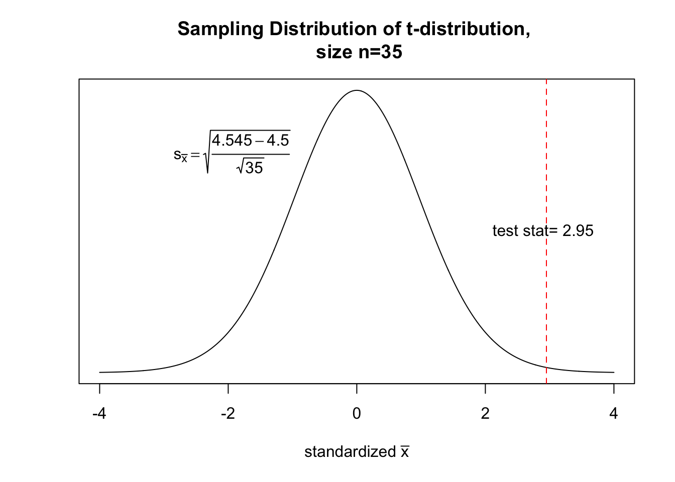
Finally, we can calculate the area beyond this test statistic, since our alternative hypothesis is \(H_a: \mu > 4.5\).
# Notice we use 1-, because this is a right-sided probability.
1- pt(2.958039892, df= 34)
## [1] 0.002815.4 Conclude
Since $ 0.01 > 0.0028$, so \(\alpha > p\), we reject \(H_0\). There is sufficient evidence that the mean length of the bolts from this manufacturer is greater than 4.5 inches.
15.5 In R
There are two approaches to this in R: either you use actual sample data, or summary statistics.
15.5.1 Using Summary Statistics
R doesn’t have a built in function that takes summary statistics, so we need to install a package called BSDA. Once you’ve loaded the library, you want to use the tsum.test() command from the package. For instructions on how to load a package, check out installing and loading packages.
##
##  One-sample t-Test
##
## data:  Summarized x
## t = 3, df = 34, p-value = 0.003
## alternative hypothesis: true mean is greater than 4.5
## 95 percent confidence interval:
##  4.511    NA
## sample estimates:
## mean of x
##     4.525
15.5.2 Using actual data
If you have actual data, use the t.test() command. Let’s say I have actual data for 35 bolts:
head(bolts)## [,1]
## [1,] 4.527
## [2,] 4.553
## [3,] 4.526
## [4,] 4.468
## [5,] 4.568
## [6,] 4.427## [1] "mean: 4.525 sd: 0.05 n: 35"
t.test(bolts,
       mu= 4.5,
       alternative="greater")
##
## One Sample t-test
##
## data: bolts
## t = 3, df = 34, p-value = 0.003
## alternative hypothesis: true mean is greater than 4.5
## 95 percent confidence interval:
## 4.511 Inf
## sample estimates:
## mean of x
## 4.525Again, regardless of whether you calculate the interval by hand, R, or the TI-84, you must complete the State, Plan, and Conclude portions as shown. Failure to do so results in lost points.