9 🔮 Linear Regression
99% of the time in Stats, you’re not just looking for an association. You want a regression line to create a linear model.
A regression line summarizes the relationship between the two variables, but only in a specific setting: when one of the variables helps explain or predict the other. Regression, unlike correlation, requires that we have an explanatory variable and a response variable.
A regression line is a model for the data, much like a sample space in our Probability unit. The equation of a regression line gives a compact mathematical description of what the model tells us between the response variable y and the explanatory variable x.
We construct a linear model using the lm command, and store it into the variable reg_line.
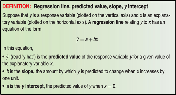
reg_line<- lm(Orange$circumference~Orange$age)If you were waiting for the regression line to suddenly appear on the scatterplot, it won’t. You must call a separate command abline(), which adds the line on top of the existing scatterplot as a new layer.
This means that you must run plot() first to create the scatterplot, and then abline() right after.
plot(y= Orange$circumference,
     x= Orange$age,
     main= "Age of Orange Trees vs. Circumference of Trunks",
     xlab= "Age of Tree (Days since Dec. 31, 1968)",
     ylab= "Trunk Circumference (mm)")

abline(reg_line, col="red")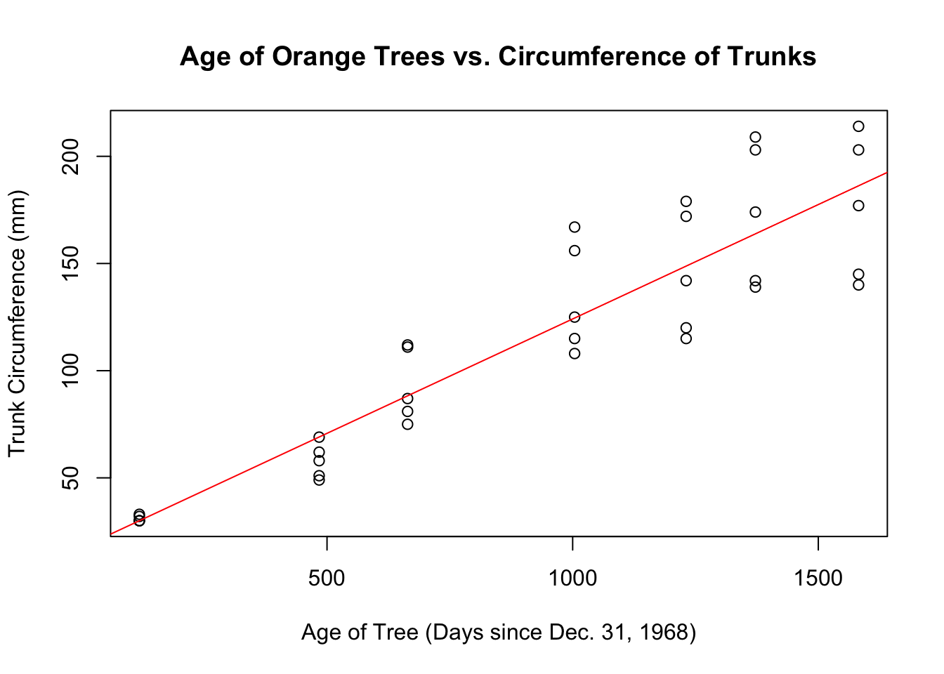
FIGURE 9.1: A Scatter Plot of Diamond Weight and Diamond Price
Like the boxplot() command in 6.4.2, the lm() command takes on two variables in the order of y~x. Be careful with placement– you always want the x variable, the explanatory variable, on the x-axis.
9.1 Create a Residual Plot
A residual is the difference between an observed (actual) value of the response variable and the predicted value by the regression line. You calculate it by: \[ \text{residual} = \text{observed y} - \text{predicted y} = y - \hat{y}\]
A residual plot takes every residual and plots it in a separate scatterplot. In effect, residual plots turn the regression line horizontal. It magnifies the deviations of the points from the line, making it easier to see unusual observations and patterns. You should always evaluate whether a linear regression line is a good fit for the model.
Whenever you create a linear model using the lm command, R automatically creates a list of residuals for you, which you plot separately.
plot(reg_line$residuals,
     ylab= "Residual",
     main= "Residual Plot for Orange Tree Regression")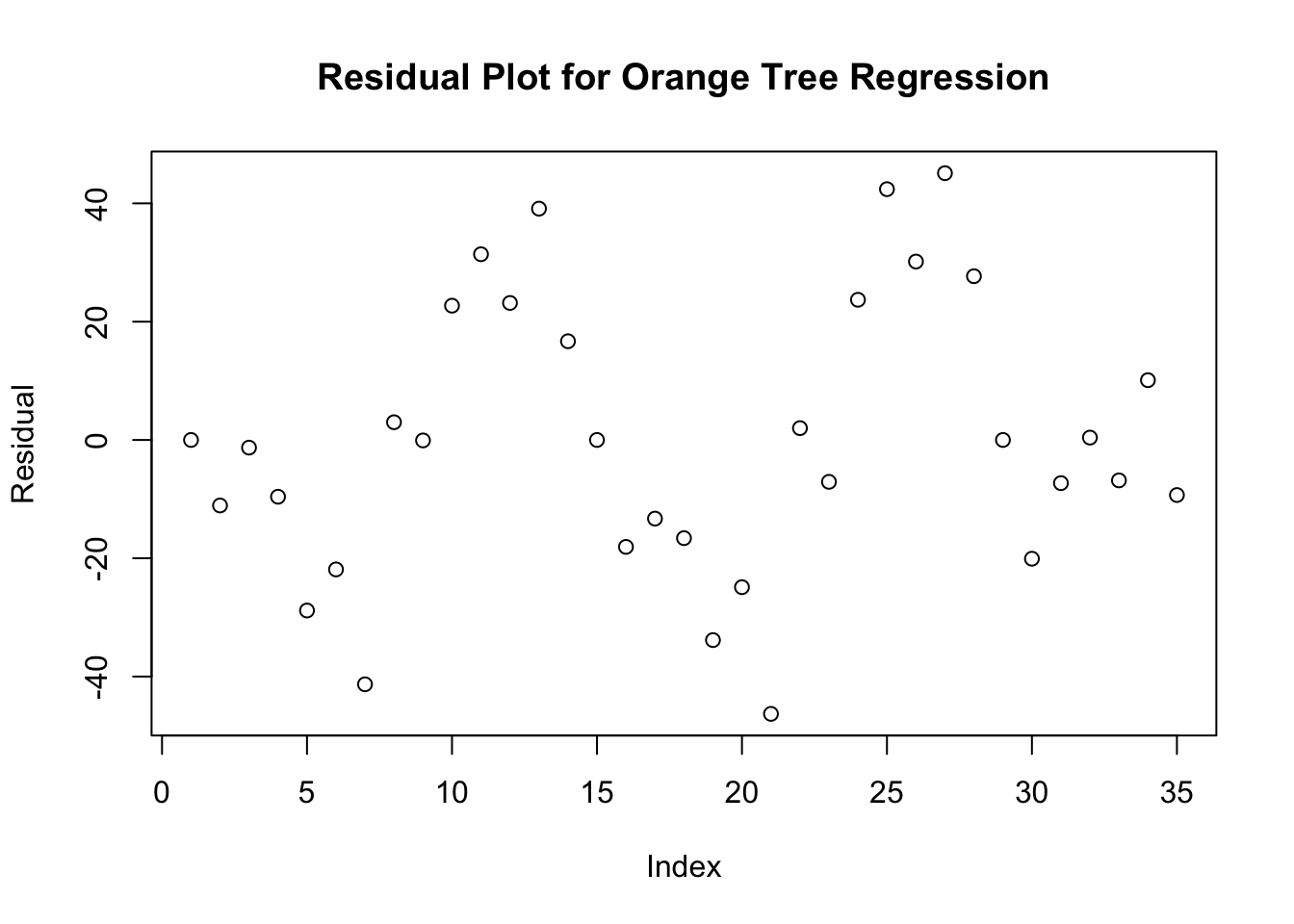
FIGURE 9.2: Resdial Plot for the Orange Tree linear model, stored as reg_line
Here are two things to look for when you examine a residual plot:
- The residual plot should show no obvious pattern. A curved pattern in a residual plot shows that the relationship is not linear. Predictions of y using this line will be less accurate for larger values of x.
- The residuals should be relatively small in size. A regression line that fits the data well should be closely “bunched” to the zero line, with no serious fan shape among the residuals.
9.2 Print Regression Output
Finally, we can get a computer printout of our regression line’s results.
summary(reg_line)##
## Call:
## lm(formula = Orange$circumference ~ Orange$age)
##
## Residuals:
## Min 1Q Median 3Q Max
## -46.31 -14.95 -0.08 19.70 45.11
##
## Coefficients:
## Estimate Std. Error t value Pr(>|t|)
## (Intercept) 17.39965 8.62266 2.02 0.052 .
## Orange$age 0.10677 0.00828 12.90 1.9e-14 ***
## ---
## Signif. codes:
## 0 '***' 0.001 '**' 0.01 '*' 0.05 '.' 0.1 ' ' 1
##
## Residual standard error: 23.7 on 33 degrees of freedom
## Multiple R-squared: 0.835, Adjusted R-squared: 0.83
## F-statistic: 166 on 1 and 33 DF, p-value: 1.93e-14By using summary, you get a computer regression printout that helps you evaluate whether the linear regression line is appropriate. The two numbers that you care about are the standard deviation of the residuals and the R-Squared Value. In R, that is labeled as Multiple R-Squared.
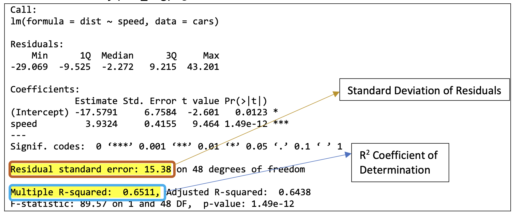
FIGURE 9.3: Interpreting a Regression Printout
A measure derived from the standard deviation of the residuals is the Coefficient of Determination, or \(R^2\).
\(R^2\) measures what proportion of our response variable’s variation (circumference) can be measured by our explanatory variable (age). In other words, what percentage of the variation in the trunk circumference of Orange trees can be explained by the age of the Orange trees?
- An \(R^2\) of 0 means that 0% of the variation of the response variable can be explained by the explanatory variable.
- An \(R^2\) of 1 means that 100% of the variation of the response variable can be explained by the explanatory variable. If every point falls directly on the LSRL, then Residual Standard Error would be 0, which means that \(R^2\) will be 1.
- Because it is a percentage, \(R^2\) can’t be negative, or greater than 1.
- Remember the correlation coefficient, r? You can calculate the correlation coefficient for any scatterplot by taking \(\sqrt{R^2}\). Incredible!
In the R Printout, ignore Adjusted R-Squared. This is for multivariable regressions, which you might learn about in RS3.
9.3 Regression Wisdom
You should never, ever, rely soley on the \(R^2\) value in order to determine whether the model is a good fit.
Anscombe’s Data (find it in R under anscombe) is a famous dataset that shows why. It is reproduced below. Read the description, and then proceed to each individual tab.
As you can see, every dataset here has the same exact r correlation coefficient, and the same \(R^2\) coefficient. However, only the first set of data is appropriate for a linear model– the other 3 are clearly not appropriate for a linear model.
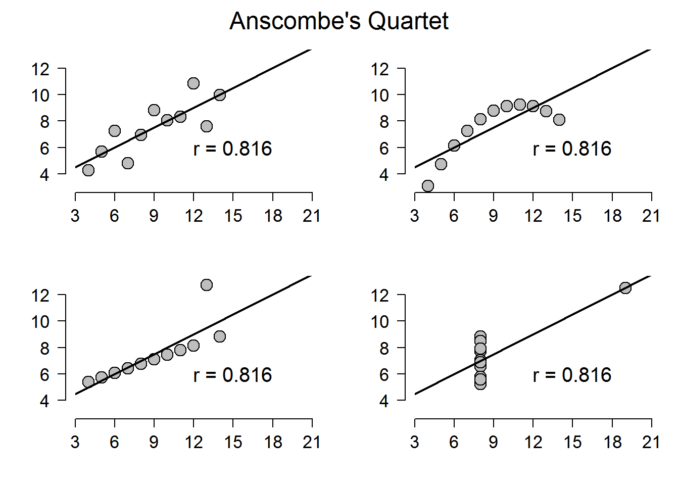
FIGURE 9.4: All four of Anscombe’s plots. Taken from https://www.shinyapps.org/apps/RGraphCompendium/index.php#anscombes-quartet
Always ask yourself these questions when you are fitting as linear model to your scatter plot:
- Are these variables quantitative?
- Is there a reasonable assumption that the two variables have a relationship with each other?
- Does the scatterplot show a reasonable strength, direction, and form?
- Does the residual plot show a reasonable scatter with no obvious pattern?
- Is the standard deviation of the residuals reasonably small?
- Is the R^2 value large?